Table of Contents
Introduction
Language used: R
Description of the dataset and variables, refer to: http://jfeggio.github.io/posts/whr1/
Goal: Identify if there is a positive correlation between the variable log_gdp and the reported happiness score (life_ladder)
Exploratory Data Analysis
Variable Life ladder among all years
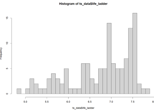
The histogram has a symmetrical distribution centered around 6.7. The majority of observations fall within the range of 6.0 to 7.5. A slight negative skewness is observed in the distribution, indicating that there are more countries with happiness levels above the average.
Variable Life ladder over the years by country
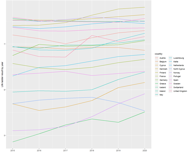
Austria shows an upward trend in happiness levels from 2015 to 2020, reaching a peak in the latter year. On the other hand, countries like Cyprus and Greece exhibit more noticeable variations in their happiness levels, with fluctuations throughout the analyzed period.
Variable freedom over the years by country
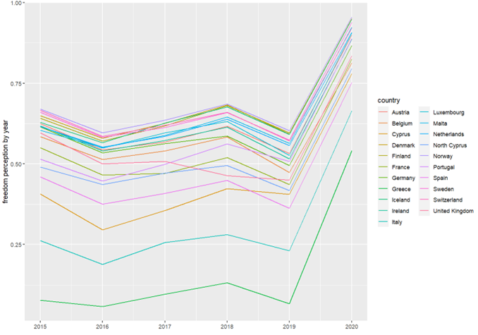
In 2015, Austria and Finland exhibit relatively high levels of freedom, while Greece and Malta have lower levels. As we progress through the years, there are fluctuations in freedom levels, but most countries seem to experience a general trend towards increased perceived freedom in 2020.
Variable perception of corruption over the years by country
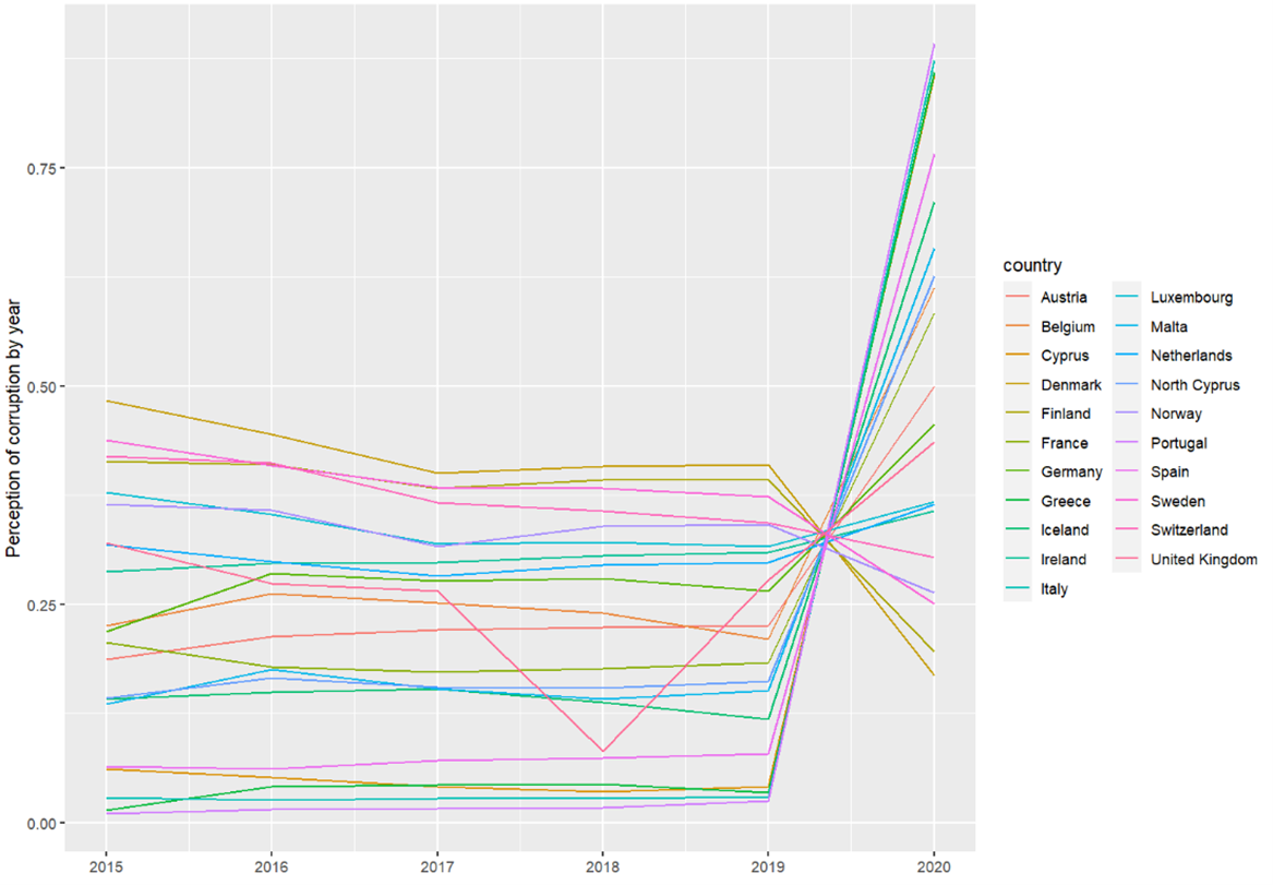
Throughout the time series, the mean of the variable perception_corruption is observed to remain at moderate levels, indicating a general perception of corruption that varies but does not significantly deviate from the average. However, the year 2020 stands out as a particularly atypical year. The same happens with the variables: social support, life expectancy, logarithm of gdp.
Preprocessing Data
Mahalanobis distance In order to detect atypical values, the mahalanobis distance is used. This calculates distance between a point and a set of points in a multivariate space, taking into account the covariance between variables. By considering covariance, the Mahalanobis distance can identify points that, although not extreme values in a single variable, are unusual in the context of the set of variables.
To apply the Mahalanobis distance, the covariance matrix and the critical value of the squared chi distribution is calculated.
Possible outliers (p-value<0.10)
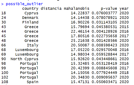
Greece, Luxembourg, and Portugal are considered as possible outliers because these are the countries that turn out to be atypical values for two or more years after graphical representation of the values over the years.
Example of detection of outliers graphs (2019) Greece=purple; Portugal=green; Luxembourg=pink
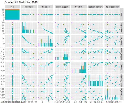
Due to Portugal and Greece frequently appearing as outliers in the visualizations, the decision is made to exclude them from the database.
Additionally, the data from 2020 will be excluded since the data was particularly atypical. The reason behind this may be related to the COVID-19 pandemic, which had a global impact on various aspects of society.
Modelling and Testing
The first step is the conversion of the database into a panel database. Then, a simple linear regression model is run with the two variables mentioned earlier to observe the situation in the year 2015.
Linear Regression Model (Year 2015)
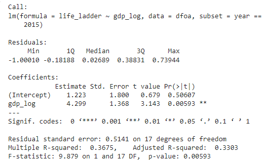
The variable gdp_log is statistically significant and positive. The expected value of life_ladder when gdp_log is zero, is 1.223, and keeping all other variables constant, there is an expected increase of 4.299 points in life_ladder for each increase in gdp_log. A similar model is created to analyze the year 2019, where no significant variations compared to the previously considered data are observed.
Linear Regression Model (Year 2019)
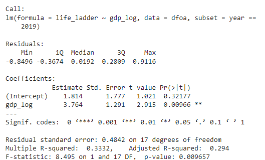
The variable gdp_log remains statistically significant and positive, confirming the initial hypothesis. The expected value of life_ladder when gdp_log is zero is 1.814, and keeping all other variables constant, there is an expected increase of 3.764 points in life_ladder for each increase in gdp_log.
Linear Regression Pooled Model (All observation)
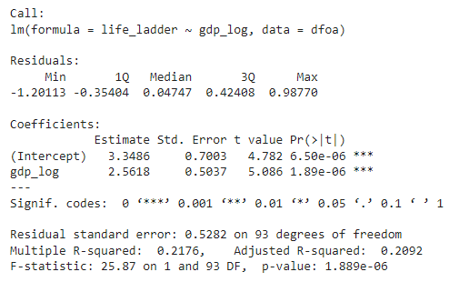
Considering all years, the variable gdp_log is even more statistically significant and maintains its positive character. The OLS linear regression models for the years considered confirm the hypothesis that the variable gdp_log is positively correlated with the variable life_ladder. It is important to highlight that there are characteristics of observations that affect the endogenous variable, not captured by the regressors and remain constant over time for each country, for example: life perspective, culture, history, etc. Therefore, it is appropriate to incorporate unobservable and constant heterogeneity over time for each of the analyzed countries.
With Wooldridge’s test of unobservable effects, the null hypothesis that there are no unobservable effects in the residual is tested. This is done to analyze whether it is preferable to use the pooled OLS model.
Wooldridge Test

In this case, the null hypothesis that there is no unobservable heterogeneity is rejected, concluding that it is not advisable to use the pooled OLS model. It is then decided to develop fixed and random effects models.
Fixed Effects Model
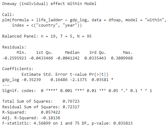
In the fixed model, unobservable heterogeneity is considered constant. The variable gdp_log remains statistically significant but becomes negative, rejecting the initial hypothesis.
Fixed Effects Model (Two Ways)
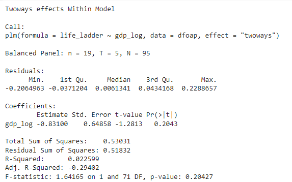
The model with fixed effects is generalized to two effects: one for individuals and one for time. In this case, the coefficient is 0.204, and it is not statistically significant. Additionally, the two-component model has a lower R-squared value compared to the one-component model. For these reasons, the one-component model is considered preferable.
To validate the choice of the fixed effects model over the pooled OLS model, the F-test is used to evaluate the existence of individual effects.
F-Test (Fixed Effects, Pooled OLS)

With the p-value less than 0.05, the null hypothesis is rejected, concluding that there are individual effects, and it is confirmed that the fixed effects model is the best choice.
Random Effects Model
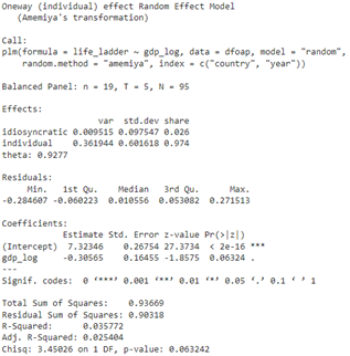
The random effects model is developed, where unobservable heterogeneity varies over time according to a certain probability distribution.
In this model, the variable gdp_log also has a negative impact but is not statistically significant in the dependent variable life_ladder. To decide which model to use, the differences between the values of both estimates are evaluated using the Hausman test.
To perform this test, the assumptions that errors are homoscedastic must be met. To verify this, the Breusch-Pagan test is used.
Breusch-Pagan Test

The p-value is greater than 0.05, meaning that the null hypothesis of no heterogeneity cannot be rejected. To consider heterogeneity values, the “aux” variant based on an auxiliary regression is added, and a robust covariance matrix is specified with the vcov argument to the Hausman test.
Hausman Test

With a p-value less than 0.05, the null hypothesis cannot be rejected, and the fixed effects estimator is preferred. This result seems reasonable, as the fixed effects model is suitable for analyzing a certain number of non-random individuals, and inference is restricted to the behavior of these individuals.
Wooldridge Test (Fixed Effects)

To detect autocorrelation, the Wooldridge test is applied to the fixed effects model. Since the p-value is less than 0.05, the null hypothesis of no serial correlation is rejected.
Unable to discard autocorrelation, the same test is applied to a model using the difference estimator.
Wooldridge Test (Differences)

In this case, the null hypothesis is also rejected, but with a p-value of 66%, which is much higher than obtained testing autocorrelation with the fixed effects model. This suggests that this model is better.
A differences model is then determined to be the most efficient model.
Differences Model
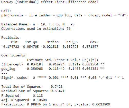
The model indicates that both the intercept and the variable gdp_log are statistically significant and have a negative impact on the dependent variable life_ladder. However, the R-squared suggests that the model explains a relatively low proportion of the variability in the dependent variable, only 11%.
The observed negative correlation may be due to various factors. An increase in GDP may occur, but it does not always translate directly into an improvement in the quality of life for all strata of society. The way in which wealth is distributed among different population segments and other related factors can influence how the increase in GDP affects happiness.
Finally, the relationship between income and happiness can be subjective and vary considerably between individuals and cultures. Some people may attribute greater value to quality of life, equality, or other non-strictly economic aspects, which can affect the perception of happiness in relation to GDP.
Conclusion
This study aimed to confirm the positive correlation between the logarithmic Gross Domestic Product (gdp_log) and the happiness score of each country (life_ladder). The initial hypothesis, suggesting a positive relationship, was rejected, as the models revealed a significant but negative relationship between the two variables. Initially, a positive and significant relationship was observed in simple linear regression models that did not consider the presence of unobservable heterogeneity.